Rapport Numerical Methods In Python

Rapport: Gauss & LU Methods In Python

Chachoua Imad Eddine, Group 3.

1. Introduction

The solution of linear systems of equations is a fundamental problem in numerical analysis, with wide applications in engineering, physics, and computer science. That’s why many techniques are used for solving such systems like Gaussian Elimination and LU Decomposition.

This document explores the concepts, algorithms, and practical applications of these methods using Python.

2. Gauss Elimination

2.1. Theory and Concept

A method of solving a linear system is as follows: Write the augmented matrix of the system, Use the elementary row operations to reduce the augmented matrix to a matrix in row-echelon form (Triangularization), Write the linear system corresponding to the row-echelon matrix and solve by back-substitution. This is known as the method of Gaussian elimination with back-substitution, in short by Gaussian elimination. It consists of two key concepts: - Triangularisation: We use elementary row operations to reduce the matrix to a matrix in row-echelon form, for example:

2. & 1. & -1. \\ 0. & 0.5 & 0.5 \\ 0. & 0. & -1. \end{bmatrix}

- Resolution: We convert the reduced matrix to a linear system, then we apply back-substitution to get the solution of the system.

2.2. Algorithm

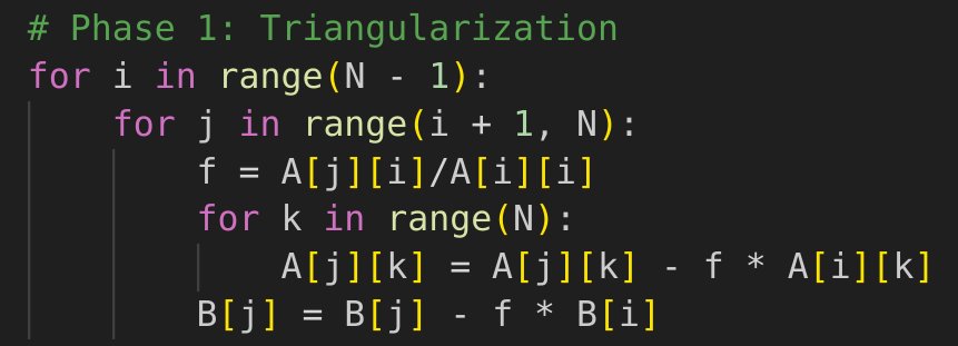
Phase 1: Triangularization

For i = 1 to N - 1
    For j = i + 1 to N
        f = A(j, i) / A(i, i)
        For k = 1 to N
            A(j, k) = A(j, k) - f * A(i, k)
        End For
        B(j) = B(j) - f * B(i)
    End For
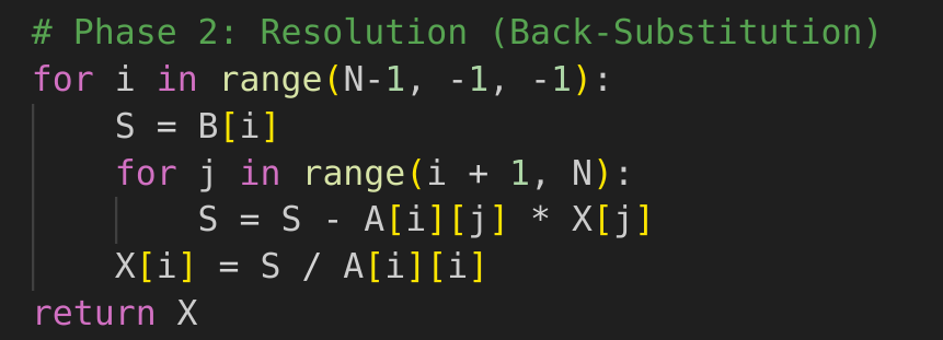
End For

Phase 2: Resolution (Back-Substitution)

For i = N to 1 step -1
    S = B(i)
    For j = i + 1 to N
        S = S - A(i, j) * X(j)
    End For
    X(i) = S / A(i, i)
End For

2.3. Implementation in Python

Phase 1: Triangularization

Phase 2: Resolution (Back-Substitution)

2.4. Practical Example

We aim to solve the following system of linear equations:

$2x_1+x_2-x_3=8$ $-3x_1-x_2+2x_3=-11$ $-2x_1+x_2+2x_3=-3$ This system can be represented in matrix form as: $AX=B$ Where: $A=\left[\begin{array}{ccc}2& 1& -1\\ -3& -1& 2\\ -2& 1& 2\end{array}\right],B=\left[\begin{array}{c}8\\ -11\\ -3\end{array}\right]$ Using Gaussian Elimination, the solution to the system above is $X=\left[\begin{array}{c}2\\ 3\\ -1\end{array}\right]$ Now let’s implement it in our code:

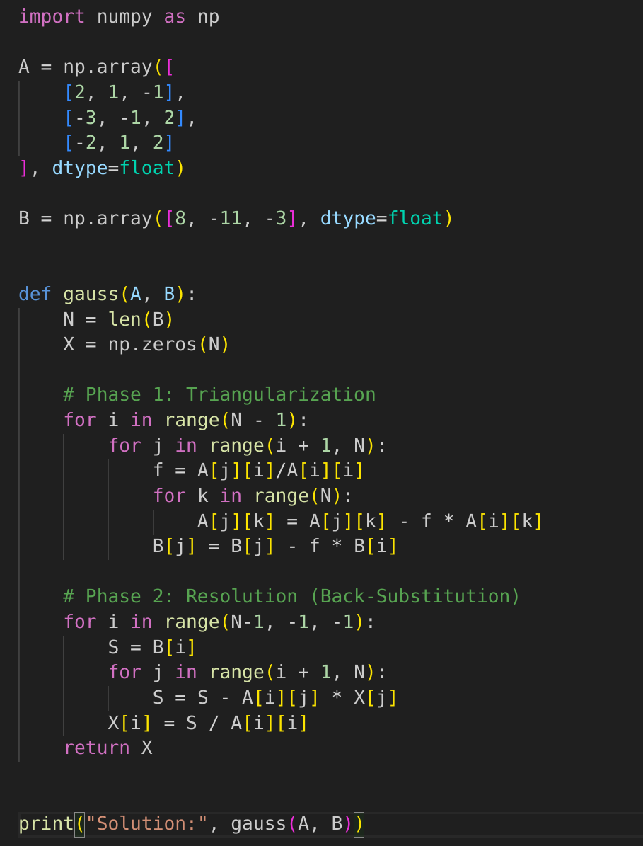
The captured output is:

2.5. Analysis of Results

The implementation of the Gauss algorithm successfully solved the given system of linear equations. After applying the triangularization method and back-substitution, the obtained solution vector is:

$$X=\left[\begin{array}{c}2\\ 3\\ -1\end{array}\right]$$

The results show that the system is well-conditioned and the algorithm converged quickly for this particular case. However, for larger or ill-conditioned systems, additional precautions (such as pivoting) may be required to improve numerical stability.

2.6. Conclusion

Our implementation of Gauss Elimination has successfully provided a solution to the system of linear equations. By analyzing the solution, we can ensure the accuracy and efficiency of the Triangularization + Resolution algorithm.

3. LU Decomposition

3.1. Theory and Concept

LU method factors a matrix into two triangular matrices, one lower triangular (L) and one upper triangular (U), enabling the solution of easy systems with shared coefficients to find the solution.

Algorithm

For i = 0 to N - 1:
    L[i][i] = 1
For i = 0 to N - 1:
    For j = i to N - 1:
        sum1 = Sum(L[i][k] * U[k][j] for k = 0 to i - 1)
        U[i][j] = A[i][j] - sum1
 
    For j = i + 1 to N - 1:
        sum2 = Sum(L[j][k] * U[k][i] for k = 0 to i - 1)
        L[j][i] = (A[j][i] - sum2) / U[i][i]
Return L, U
 

3.2. Implementation in Python

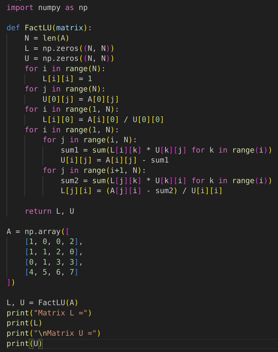
3.3. Practical Examples

We aim to decompose the following matrices:

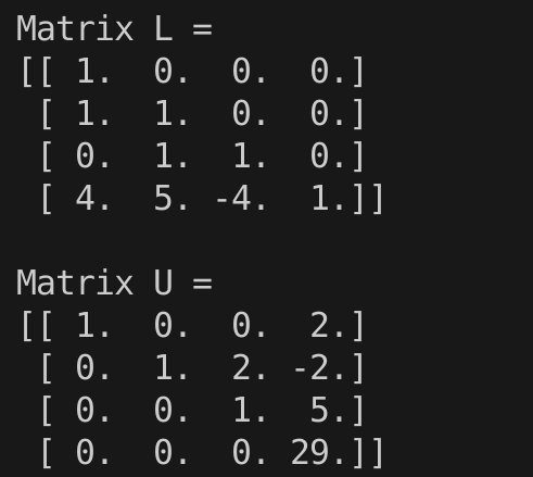
$A=\left[\begin{array}{cccc}1& 0& 0& 2\\ 1& 1& 2& 0\\ 0& 1& 3& 3\\ 4& 5& 6& 7\end{array}\right],B=\left[\begin{array}{cccc}1& 0& 0& 2\\ 1& 0& 2& 0\\ 0& 1& 3& 3\\ 4& 5& 6& 7\end{array}\right]$ The solution should be: for A: $L=\left[\begin{array}{cccc}1& 0& 0& 0\\ 1& 1& 0& 0\\ 0& 1& 1& 0\\ 4& 5& 6& 1\end{array}\right],U=\left[\begin{array}{cccc}1& 0& 0& 2\\ 0& 1& 2& -2\\ 0& 0& 3& 3\\ 0& 0& 0& 7\end{array}\right]$ for B: $L=\left[\begin{array}{cccc}1& 0& 0& 0\\ -1& 1& 0& 0\\ 0& -0.5& 1& 0\\ -4& -2.5& -2& 1\end{array}\right],U=\left[\begin{array}{cccc}-1& 0& 0& 2\\ 0& -2& 0& 2\\ 0& 0& -3& 4\\ 0& 0& 0& 7\end{array}\right]$ The captured output: for A: for B:

3.4. Analysis of results

The LU decomposition method successfully factorizes the matrix A into L and U with LU = A. While it shows an error doing the same with matrix B, as it encountered a division by zero.

3.5. Conclusion

The LU decomposition method successfully factorizes the matrix A into L and U. By solving LY = B and UX=Y, we will efficiently obtain the solution vector. The results confirm the correctness and of LU decomposition for this specific system. However, for or ill-conditioned matrices like B, A division by zero error has occurred, thus, numerical pivoting might be necessary.

4. Conclusion

Gaussian Elimination and LU Decomposition are powerful tools for solving systems of linear equations. The implementation of Gaussian Elimination demonstrates the reduction of a matrix to row-echelon form, followed by back-substitution to determine the solution. The LU decomposition method simplifies the process by decomposing the matrix into L and U matrices, facilitating the solution of the systems By solving LY = B and UX=Y.

However, while these methods are effective, their effectiveness can be limited in some cases, that’s why a technique like pivoting and other stability-improving techniques are used to improve its efficiency.